Kernels
A memory kernel kernel is an instance of a type of which MemoryKernel is a supertype. It can be used to compute out = evaluate_kernel(kernel, F, t) to find the value of the memory kernel. Additionally, when F is a mutable container like a Vector, one can call evaluate_kernel!(out, kernel, F, t) in which case it will mutate the elements of the temporary array out. Below we list the memory kernels that this package defines and give some examples of how to use them.
Schematic Kernels
This package includes a couple of schematic memory kernels.
ExponentiallyDecayingKernel
The ExponentiallyDecayingKernel implements the kernel $K(t) = λ \exp(-t/τ)$. It has fields λ <: Number and τ <: Number.
Example
The integrodifferential equation with this memory kernel has an analytic solution for $\tau=1$, $\alpha=0$ , $\beta=1$, and $\gamma=1$. It is given by
\[F(t) = \frac{e^{-\frac{t}{2}\left( \lambda + \sqrt{\lambda(\lambda+4)} + 2\right)}}{2 \sqrt{\lambda (\lambda +4)}}\left(\sqrt{\lambda(\lambda+4)} \left(e^{\sqrt{\lambda(\lambda+4)} t}+1\right)+\lambda \left(e^{\sqrt{\lambda(\lambda+4)} t}-1\right)\right)\]
F0 = 1.0; ∂F0 = 0.0; α = 0.0; β = 1.0; γ = 1.0; δ = 0.0; λ = 1.0; τ = 1.0;

kernel = ExponentiallyDecayingKernel(λ, τ)
problem = MemoryEquation(α, β, γ, δ, F0, ∂F0, kernel)
solver = TimeDoublingSolver(Δt=10^-3, t_max=10.0^2, verbose=false, N = 128, tolerance=10^-10, max_iterations=10^6)
sol =  solve(problem, solver)

t_analytic = 10 .^ range(-3, 2, length=50)
F_analytic = @. (exp(-0.5*(3+sqrt(5))* t_analytic)*(exp(sqrt(5)*t_analytic) * (1+sqrt(5))-1+sqrt(5)))/(2sqrt(5))

using Plots
p = plot(log10.(get_t(sol)), get_F(sol), label="Numeric solution", lw=3)
scatter!(log10.(t_analytic), F_analytic, label="Exact solution", ylabel="F", xlabel="log10(t)")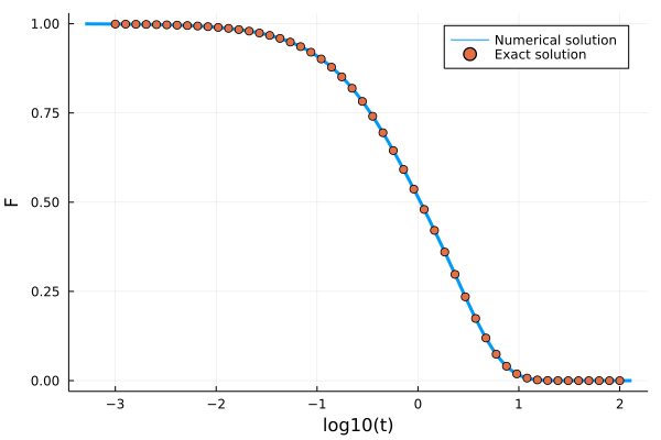
SchematicF1Kernel
The SchematicF1Kernel implements the kernel $K(t) = ν F(t)$. It has one field ν <: Number.
Example
The integro-differential equation with this memory kernel also has an analytic solution for $\alpha=0$ , $\beta=1$, and $\nu=1$. It is given by
\[F(t) = e^{-2t}\left(I_0(2t) + I_1(2t) \right)\]
in which $I_k$ are modified Bessel functions of the first kind.
F0 = 1.0; ∂F0 = 0.0; α = 0.0; β = 1.0; γ = 1.0; ν = 1.0; δ = 0.0

kernel = SchematicF1Kernel(ν)
problem = MemoryEquation(α, β, γ, δ, F0, ∂F0, kernel)
solver = TimeDoublingSolver(Δt=10^-3, t_max=10.0^2, verbose=false, N = 100, tolerance=10^-14, max_iterations=10^6)
sol =  solve(problem, solver)

using Plots, SpecialFunctions
t_analytic = 10 .^ range(-3, 2, length=50)
F_analytic = @. exp(-2*t_analytic)*(besseli(0, 2t_analytic) + besseli(1, 2t_analytic))
plot(log10.(get_t(sol)), get_F(sol), label="Numerical Solution", ylabel="F", xlabel="log10(t)", lw=3)
scatter!(log10.(t_analytic), F_analytic, label="Exact Solution")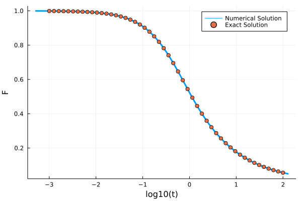
SchematicF2Kernel
The SchematicF2Kernel implements the kernel $K(t) = ν F(t)^2$. It has one field ν <: Number.
SchematicF123Kernel
The SchematicF123Kernel implements the kernel $K(t) = \nu_1 F(t) + \nu_2 F(t)^2 + \nu_3 F(t)^3$. It has fields ν1 <: Number, ν2 <: Number, and ν3 <: Number.
Example
kernel = SchematicF123Kernel(3.0, 2.0, 1.0);
F = 2; t = 0;
evaluate_kernel(kernel, F, t) # returns 22.0 = 3*2^1 + 2*2^2 + 1*2^3
InterpolatingKernel
The InterpolatingKernel implements a kernel that interpolates memory kernel data. It is initialized by calling kernel = InterpolatingKernel(t, M, k=k) where t is a Vector of time points, M is a vector of corresponding memory kernel values, and k is the integer degree of polynomial interpolation (default=1). This kernel is implemented using Dierckx.Spline1D. See Dierckx.jl for more information.
SchematicDiagonalKernel
The SchematicDiagonalKernel implements the kernel $K_{ij}(t) = \delta_{ij} \nu_i F_i(t)^2$. It has one field ν which must be either a Vector or an SVector. When called, it returns Diagonal(ν .* F .^ 2), i.e., it implements a non-coupled system of SchematicF2Kernels.
SchematicMatrixKernel
The SchematicMatrixKernel implements the kernel $K_{ij}(t) = \sum_k \nu_{ij} F_k(t) F_j(t)$. It has one field ν which must be either a Matrix or an SMatrix.
SjogrenKernel
The SjogrenKernel implements the kernel $K_{1}(t) = \nu_1 F_1(t)^2$, $K_{2}(t) = \nu_2 F_1(t) F_2(t)$. It has two fields ν1 and ν2 which must both be of the same type. Consider using Static Vectors for performance.
Example:
using StaticArrays
α = 1.0
β = 0.0
γ = 1.0
δ = 0.0
ν1 = 2.0
ν2 = 1.0
F0 = @SVector [1.0, 1.0]
∂F0 = @SVector [0.0, 0.0]
kernel = SjogrenKernel(ν1, ν2)
eq = MemoryEquation(α, β, γ, δ, F0, ∂F0, kernel)
sol = solve(eq)
TaggedSchematicF2Kernel
The TaggedSchematicF2Kernel implements a memory kernel $K(t) = \nu F(t) F_c(t)$, where $F_c(t)$ is a correlator that the tagged one couples to. It must be a solution of an earlier schematic MCT equation. Make sure to use the same solver settings for both solutions.
Example:
F0 = 1.0
∂F0 = 0.0
α = 1.0
β = 0.0
γ = 1.0
δ = 0.0
ν1 = 2.0
ν2 = 1.0
kernel = SchematicF2Kernel(ν1)
eq = MemoryEquation(α, β, γ, δ, F0, ∂F0, kernel)
sol = solve(eq)

taggedkernel = TaggedSchematicF2Kernel(ν2, sol)
tagged_eq = MemoryEquation(α, β, γ, δ, F0, ∂F0, taggedkernel)
tagged_sol = solve(tagged_eq);
This example is (less performantly) equivalent to the example of the Sjogren kernel above.
Mode-Coupling Kernel
See the next page of the documentation for information on the kernels for mode-coupling theory.
Defining custom kernels
In order to define a custom kernel, one has to overload ModeCouplingTheory.evaluate_kernel(k::MyCustomKernel, F, t), and optionally ModeCouplingTheory.evaluate_kernel!(out, k::MyCustomKernel, F, t) for better performance for mutable F.
Example 1
Let's define a custom scalar kernel that evaluates $K(t) = \alpha F(t)^{F(t)}$. First, we define a MyWeirdKernel<:MemoryKernel type that holds the value of the parameter:
using ModeCouplingTheory
import ModeCouplingTheory.MemoryKernel

struct MyWeirdKernel <: MemoryKernel
    α :: Float64
end

kernel = MyWeirdKernel(2.5)
Now, we can define the evaluation of this memory kernel
import ModeCouplingTheory.evaluate_kernel

function evaluate_kernel(kernel::MyWeirdKernel, F, t)
    return kernel.α*F^F
end
That's it! We can now use it like any other memory kernel to solve the equation:
problem = MemoryEquation(1.0, 0.0, 1.0, 0.0, 1.0, 0.0, kernel)
solver = TimeDoublingSolver(Δt = 10^-4, t_max=10.0^5)
sol = solve(problem, solver)
using Plots
p = plot(log10.(sol.t), sol.F, ylims=(0,1), ylabel="F(t)", xlabel="log10(t)")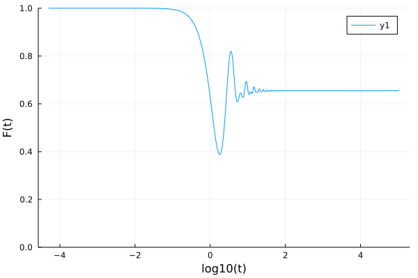
Example 2
For a slightly more complex example, let's define the mode-coupling theory memory kernel (say we forgot that it is also a built-in kernel). The equation is given by:
\[\ddot{F}(k,t) + \frac{k^2 k_BT}{m S(k)} F(k,t) + \int_0^t d\tau K(k, t-\tau)\dot{F}(k, \tau)=0,\]
in which
\[K(k,t) = \frac{\rho k_BT}{16\pi^3 m} \int d\mathbf{q} V(\mathbf{k}, \mathbf{q})^2F(q, t)F(|\mathbf{k}-\mathbf{q}|,t)\]
where
\[V(\textbf{k}, \textbf{q}) = (\textbf{k}\cdot\textbf{q})c(q)/k+(\textbf{k}\cdot(\textbf{k}-\textbf{q})c(|\textbf{k}-\textbf{q}|)/k,\]
where $p = |\textbf{k} - \textbf{q}|$. For more information, see the next page of the docs, which is dedicated to this equation.
First, we need to evaluate the structure factor, and some input parameters:
using ModeCouplingTheory, LinearAlgebra

"""
    find_analytical_C_k(k, η)
Finds the direct correlation function given by the
analytical Percus-Yevick solution of the Ornstein-Zernike
equation for hard spheres for a given volume fraction η.

Reference: Wertheim, M. S. "Exact solution of the Percus-Yevick integral equation
for hard spheres." Physical Review Letters 10.8 (1963): 321.
"""
function find_analytical_C_k(k, η)
    A = -(1 - η)^-4 *(1 + 2η)^2
    B = (1 - η)^-4*  6η*(1 + η/2)^2
    D = -(1 - η)^-4 * 1/2 * η*(1 + 2η)^2
    Cₖ = @. 4π/k^6 *
    (
        24*D - 2*B * k^2 - (24*D - 2 * (B + 6*D) * k^2 + (A + B + D) * k^4) * cos(k)
     + k * (-24*D + (A + 2*B + 4*D) * k^2) * sin(k)
     )
    return Cₖ
end

"""
    find_analytical_S_k(k, η)
Finds the static structure factor given by the
analytical Percus-Yevick solution of the Ornstein-Zernike
equation for hard spheres for a given volume fraction η.
"""
function find_analytical_S_k(k, η)
        Cₖ = find_analytical_C_k(k, η)
        ρ = 6/π * η
        Sₖ = @. 1 + ρ*Cₖ / (1 - ρ*Cₖ)
    return Sₖ
end
η = 0.5158; ρ = η*6/π; kBT = 1.0; m = 1.0

Nk = 100; kmax = 40.0; dk = kmax/Nk; k_array = dk*(collect(1:Nk) .- 0.5)
Sₖ = find_analytical_S_k(k_array, η)
Cₖ = find_analytical_C_k(k_array, η)
∂F0 = zeros(Nk); α = 1.0; β = 0.0; γ = @. k_array^2*kBT/(m*Sₖ); δ = 0.0
Now, we need to construct the memory kernel for the intermediate scattering function F. For performance reasons, we also implement the in-place evaluate_kernel!(out, kernel, Fs, t). The discrete equation that we must implement is given by
\[K(k_i,t) = \frac{\rho k_BT \Delta k^2}{8\pi^2 m}\sum_{j=1}^{N_k} \sum_{l=|j-i|+1}^{j+i-1} \frac{p_l q_j}{k_i}F(q_j)F(p_l)V^2(k_i, q_j, p_l).\]
This memory kernel can now be straightforwardly implemented as follows:
import ModeCouplingTheory.MemoryKernel
struct MCTKernel <: MemoryKernel
    V²::Array{Float64, 3}
    k_array::Vector{Float64}
    prefactor::Float64
end

# The constructor for the MCTKernel
function MCTKernel(ρ, kBT, m, k_array, Cₖ)
    Δk = k_array[2] - k_array[1]
    prefactor = ρ*kBT*Δk^2/(8*π^2*m)
    Nk = length(k_array)
    # calculate the vertices
    V² = zeros(Nk, Nk, Nk)
    for i = 1:Nk, j = 1:Nk, l = 1:Nk # loop over k, q, p
        k = k_array[i]
        q = k_array[j]
        p = k_array[l]
        cq = Cₖ[j]
        cp = Cₖ[l]
        if abs(j-i)+1 <= l <= j+i-1
            V = cq * (k^2  + q^2 - p^2)/(2k) + cp * (k^2  + p^2 - q^2)/(2k)
            V²[l, j, i] = V^2
        end
    end
    return MCTKernel(V², k_array, prefactor)
end
Now to evaluate the kernel, we first write the in-place version of the code, that mutates its first argument. Note also that, since the mermory kernel is multiplied with a vector F to produce something of the same type of F, it has to be encoded as a matrix, with on the diagonal the discretised wave-number dependent memory kernel values.
import ModeCouplingTheory.evaluate_kernel!
function evaluate_kernel!(out::Diagonal, kernel::MCTKernel, F, t)
    out.diag .= zero(eltype(out.diag)) # set the output array to zero
    k_array = kernel.k_array
    Nk = length(k_array)
    for i = 1:Nk, j = 1:Nk, l = 1:Nk # loop over k, q, p
        k = k_array[i]
        q = k_array[j]
        p = k_array[l]
        out.diag[i] += p*q/k * kernel.V²[l, j, i] * F[j] * F[l]
    end
    out.diag .*= kernel.prefactor
end

import ModeCouplingTheory.evaluate_kernel
function evaluate_kernel(kernel::MCTKernel, F, t)
    out = Diagonal(similar(F)) # we need it to produce a diagonal matrix
    evaluate_kernel!(out, kernel, F, t) # call the inplace version
    return out
end
Now we can solve the equation:
kernel = MCTKernel(ρ, kBT, m, k_array, Cₖ);
equation = MemoryEquation(α, β, γ, δ, Sₖ, ∂F0, kernel);
solver = TimeDoublingSolver(Δt=10^-5, t_max=10.0^10,
N = 8, tolerance=10^-8, verbose=true);
sol = @time solve(equation, solver);
using Plots
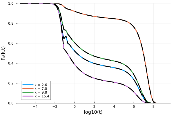
p = plot(xlabel="log10(t)", ylabel="Fₛ(k,t)", ylims=(0,1))
for ik = [7, 18, 25, 39]
Fk = get_F(sol, 1:10:800, ik)
t = get_t(sol)[1:10:800]
plot!(p, log10.(t), Fk/Sₖ[ik], label="k = $(k_array[ik])", lw=3)
end
pThis implementation of the memory kernel is much slower than the built-in one, and can be made much more performant by Bengtzelius' trick. For the purposes of this example, however, we do not pursue this any further. For help with implementing your own kernel, please file an issue.
We can verify that the results are the same with the built-in memory kernel:
kernel2 = ModeCouplingKernel(ρ, kBT, m, k_array, Sₖ);
equation2 = MemoryEquation(α, β, γ, δ, Sₖ, ∂F0, kernel2);
sol2 = @time solve(equation2, solver);

for ik = [7, 18, 25, 39]
    Fk = get_F(sol2, 1:10:800, ik)
    t = get_t(sol2)[1:10:800]
    plot!(p, log10.(t), Fk/Sₖ[ik], label=false, lw=3, ls=:dash, c=:black)
end
p