Time-dependent coefficients

In order to allow the coefficients $\alpha$, $\beta$, $\gamma$, and $\delta$ to have a time dependence, the constructor of MemoryEquation allows for an optional keyword argument update_coefficients!, which should be a user-defined function that updates the coefficient struct given a value of t. Make sure, when updating the coefficients, that their type does not change. The type of the coefficients can be inspected in the coeffs field of a MemoryEquation object.

The default is that all coefficients are independent of time, that is: update_coefficients! = (coeffs, t) -> nothing.

Example

Let's say we want the coefficient γ to be equal to $2 + \cos(\sqrt(t))$, this can be achieved like this:

α=1.0, β=0.0, γ=3.0, δ=0.0; F0=1.0; dF0=0.0
kernel = SchematicF2Kernel(3.9)

function myfunc(coeffs, t)
    coeffs.γ = 2+cos(sqrt(t))
end

MemoryEquation(α, β, γ, δ, F0, ∂F0, kernel; update_coefficients! = myfunc)

Alternatively, let's say we want to solve $\ddot{F} + F - t = 0$, which has the analytical solution $F(t) = t + \cos(t) - \sin(t)$

import ModeCouplingTheory: MemoryKernel, evaluate_kernel
function myfunc(coeffs, t)
    coeffs.δ = -t
end
struct ZeroKernel <: MemoryKernel end
evaluate_kernel(::ZeroKernel, _, _) = 0.0
α = 1.0; β = 0.0; γ = 1.0; δ = 0.0; F0 = 1.0; dF0 = 0.0; kernel = ZeroKernel()
equation = MemoryEquation(α, β, γ, δ, F0, dF0, kernel; update_coefficients! = myfunc)
solver = TimeDoublingSolver(t_max = 10.0^3, N = 600, Δt = 10^-4)
sol = solve(equation, solver)
t = sol.t; F = sol.F
plot(log10.(t), log10.(F), lw=3)
plot!(log10.(t), log10.(t .+ cos.(t) .- sin.(t)), ls=:dash, lw=3)

Automatic differentiation

This package is compatible with forward-mode automatic differentiation. This makes it possible to calculate quantities such as $\frac{dF(t)}{d\lambda}$ for example, where $\lambda$ is a parameter of the memory kernel.

Example

Let's take the derivative of the solution to the generalized Langevin equation with the exponentially decaying kernel with respect to the coupling parameter. First, we need to write a function that solves this equation and outputs the solution for a given coupling parameter. Since we know the analytical solution, we can compare it with the derivative of that.

using ModeCouplingTheory, Plots
function my_func(λ)
    F0 = 1.0
    ∂F0 = 0.0
    α = 0.0
    β = 1.0
    γ = 1.0
    δ = 0.0
    kernel = ExponentiallyDecayingKernel(λ, 1.0)
    problem = MemoryEquation(α, β, γ, δ, F0, ∂F0, kernel)
    solver = TimeDoublingSolver(Δt=10^-4, t_max=5*10.0^1, verbose=false, N = 128, tolerance=10^-10, max_iterations=10^6)

    sol =  solve(problem, solver)
    return sol
end

function exact_func(λ, t)
    temp = sqrt(λ*(λ+4)) 
    F = @. exp(-0.5* t*(temp+λ+2)) * (temp*(exp(temp*t)+1)+ λ* (exp(temp*t)-1)) / (2temp) 
    return [t, F]
end

sol = my_func(5.0)
texact, Fexact = exact_func(5.0, t)

p = plot(log10.(texact), Fexact, label="Exact", lw=4) 
scatter!(log10.(sol.t[1:100:end]), sol.F[1:100:end], label="Numerical solution", ls=:dash, lw=4)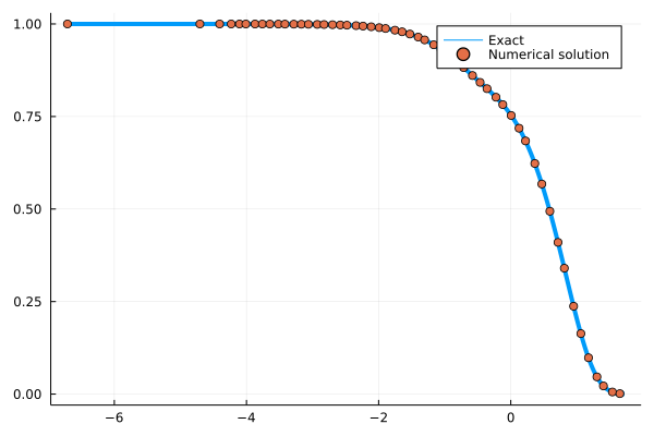 

Now we can take the derivative with respect to the argument of the functions we defined:

using ForwardDiff
_, dF_exact = ForwardDiff.derivative(y -> exact_func(y, t), 5.0)
sol = ForwardDiff.derivative(my_func, 5.0)

p = plot(log10.(texact), dF_exact, lw=3, label="Exact", ylabel="dF/dλ(λ=5,t)", xlabel="log10(t)") 
plot!(log10.(sol.t), sol.dF, ls=:dash, lw=3, label="Numerical solution", legend=:topleft)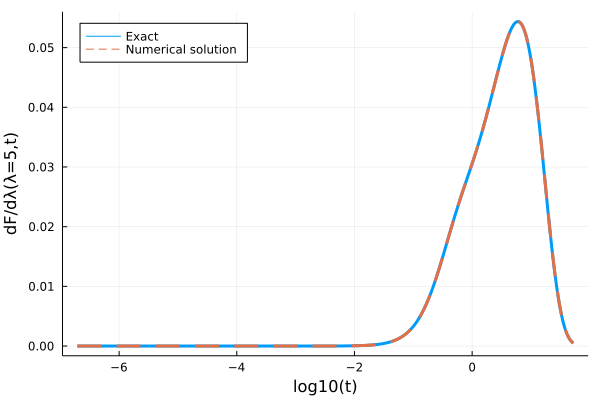

Measurement errors and other number types

Similar to automatically evaluating derivatives, it is also possible to automatically propagate measurement errors through the entire solution process. This does however cause a serious performance loss. It works by instead of doing arithmetic with standard floating point numbers, it uses numbers with an error attached. The Measurements.jl package implements how arithmetic with such numbers should be performed. Analogously, one can use arbitrary precision arithmetic (when many decimal places of precision are required) or complex-valued numbers together with this package.

Example

Let's solve standard mode-coupling theory with a structure factor that contains measurement errors. To generate such a structure factor, we can use the analytical Percus-Yevick expression, but pretend there is an uncertainty in the volume fraction $\eta$.

julia> using ModeCouplingTheory, Plots, Measurements

julia> η = 0.51 ± 0.01
0.51 ± 0.05

julia> ρ = η*6/π
0.974 ± 0.019

julia> kBT = 1.0; m = 1.0;

julia> Nk = 100; kmax = 40.0; dk = kmax/Nk; k_array = dk*(collect(1:Nk) .- 0.5);

We use the same functions to find the structure factor as before:

"""
Finds the Fourier transform of the direct correlation function given by the 
analytical Percus-Yevick solution of the Ornstein Zernike 
equation for hard spheres for a given volume fraction η on the coordinates r
in units of one over the diameter of the particles
""" 
function find_analytical_C_k(k, η)
    A = -(1 - η)^-4 *(1 + 2η)^2
    B = (1 - η)^-4*  6η*(1 + η/2)^2
    D = -(1 - η)^-4 * 1/2 * η*(1 + 2η)^2
    Cₖ = @. 4π/k^6 * 
    (
        24*D - 2*B * k^2 - (24*D - 2 * (B + 6*D) * k^2 + (A + B + D) * k^4) * cos(k)
     + k * (-24*D + (A + 2*B + 4*D) * k^2) * sin(k)
     )
    return Cₖ
end

"""
Finds the static structure factor given by the 
analytical Percus-Yevick solution of the Ornstein Zernike 
equation for hard spheres for a given volume fraction η on the coordinates r
in units of one over the diameter of the particles
""" 
function find_analytical_S_k(k, η)
        Cₖ = find_analytical_C_k(k, η)
        ρ = 6/π * η
        Sₖ = @. 1 + ρ*Cₖ / (1 - ρ*Cₖ)
    return Sₖ
end

julia> Sₖ_uncertain = find_analytical_S_k(k_array, ρ*π/6)
100-element Vector{Measurement{Float64}}:
  0.0142 ± 0.0014
  0.0145 ± 0.0015
  0.0152 ± 0.0015
  0.0163 ± 0.0017
         ⋮
  1.0154 ± 0.0012
  0.9987 ± 0.00012
 0.98327 ± 0.00089

julia> plot(k_array, Sₖ_uncertain, xlabel="k", ylabel="S(k)", legend=false)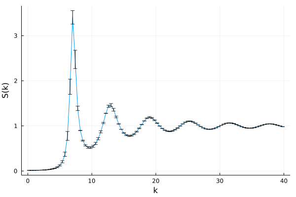

Now we can use this structure factor to solve the mode-coupling equation as usual.

# The initial condition of the derivative must have the same type as the initial condition itself
∂F0 = zeros(eltype(Sₖ_uncertain), Nk)
α = 1.0; β = 0.0; γ = @. k_array^2*kBT/(m*Sₖ_uncertain); δ = 0.0
kernel = ModeCouplingKernel(ρ, kBT, m, k_array, Sₖ_uncertain)
problem = MemoryEquation(α, β, γ, δ, Sₖ_uncertain, ∂F0, kernel)
solver = TimeDoublingSolver(Δt=10^-5, t_max=10.0^5, verbose=true, N = 8, tolerance=10^-8, max_iterations=10^8)
sol = @time solve(problem, solver);
p = plot(xlabel="log10(t)", ylabel="F(k,t)", ylims=(0,1), xlims=(-5,5))
plot!(p, log10.(get_t(sol)[2:10:end]), get_F(sol, :, 19)/Sₖ_uncertain[19], label="k = $(k_array[19])", lw=3)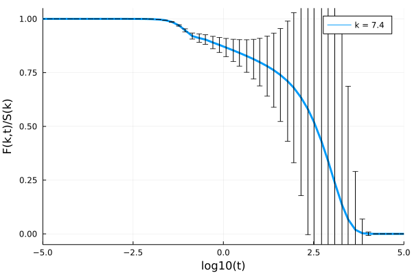

Steady state (non-ergodicity parameter)

This package also exports a function solve_steady_state(γ, F₀, kernel; tolerance=10^-8, max_iterations=10^6, verbose=false) to find the steady-state solution of a mode-coupling-like equation. In order to find it, it performs a recursive iteration of the mapping

\[F^\infty = (K(F^\infty,t=\infty) + γ)^{-1} \cdot K(F^\infty, t=\infty) \cdot F(t=0)\]

It returns a MemoryEquationSolution object defined at one time $t=\infty$, which contains both $F(t=\infty)$ and $K(t=\infty)$ as fields.

Example

using ModeCouplingTheory, Plots
η = 0.51595; ρ = η*6/π; kBT = 1.0; m = 1.0
Nk = 100; kmax = 40.0; dk = kmax/Nk; k_array = dk*(collect(1:Nk) .- 0.5);
Sₖ = find_analytical_S_k(k_array, ρ*π/6)

γ = @. k_array^2*kBT/(m*Sₖ)
kernel = ModeCouplingKernel(ρ, kBT, m, k_array, Sₖ)
sol = solve_steady_state(γ, Sₖ, kernel; tolerance=10^-8, verbose=false)
fk = get_F(sol, 1, :)
p = plot(k_array, fk, ylabel="non-ergodicity parameter", xlabel="k")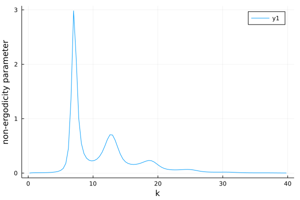

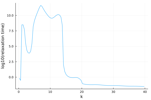
Relaxation time

Relaxation times can be easily extracted from dynamical data using the find_relaxation_time(t, F; threshold=exp(-1), mode=:log) function.

Example

Let's solve mode-coupling theory to get some data:

# We solve MCT for hard spheres at a volume fraction of 0.51591
η = 0.51591; ρ = η*6/π; kBT = 1.0; m = 1.0

Nk = 100; kmax = 40.0; dk = kmax/Nk; k_array = dk*(collect(1:Nk) .- 0.5)
Sₖ = find_analytical_S_k(k_array, η)

∂F0 = zeros(Nk); α = 1.0; β = 0.0; γ = @. k_array^2*kBT/(m*Sₖ); δ = 0.0

kernel = ModeCouplingKernel(ρ, kBT, m, k_array, Sₖ)
problem = MemoryEquation(α, β, γ, δ, Sₖ, ∂F0, kernel)
solver = TimeDoublingSolver(Δt=10^-5, t_max=10.0^15, verbose=false, 
                     N = 8, tolerance=10^-8)
sol = @time solve(problem, solver);

We can now extract a single relaxation time by calling

julia> find_relaxation_time(get_t(sol), get_F(sol, :, 18)) # at k k_array[18]
4.232796654132995e11

To extract all relaxation times as a function of $k$:

julia> t_R = [find_relaxation_time(get_t(sol), get_F(sol, :, ik)) for ik in eachindex(k_array)]; 
julia> p = plot(k_array, log10.(t_R), xlabel="k", ylabel="log10(relaxation time)", legend=false)